A Sliced Learning Framework for Online Disturbance Identification in Quadrotor SO(3) Attitude Control

Why Sliced Learning?

The central idea is simple: do not ask one opaque, high-dimensional network to rediscover the geometry of rotation. Expose that geometry first, then let three compact learners adapt inside the natural body-axis subspaces.

Conventional neural augmentation often learns from rotational states such as Euler angles. Those coordinates are intuitive, but they introduce singularities and can obscure the intrinsic structure of the rotation manifold. Sliced Learning instead adopts learning from error: it uses the Lie-algebraic attitude and angular-velocity errors already produced by geometric control.

Because the Lie algebra satisfies $\mathfrak{so}(3)\cong\mathbb{R}^3$, the rotational mismatch becomes a three-component Euclidean vector without abandoning the underlying $\mathrm{SO}(3)$ geometry. Each component defines an axis-aligned subspace in which a small adaptive learner can run independently and in parallel.

Conventional

Learning from states

Euler or coordinate-dependent inputs
Coupled high-dimensional mapping
Monolithic adaptation and tuning
Geometry must be relearned from data

Sliced Learning

Learning from geometric error

Intrinsic Lie-algebraic inputs
Three low-dimensional mappings
Independent, axis-wise adaptation
$\mathrm{SO}(3)$ structure is preserved

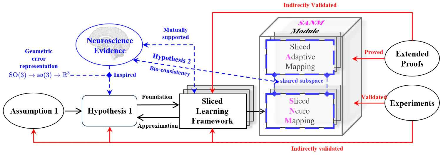
Conceptual roadmap from geometric errors and neuroscience evidence to Sliced Learning, SANM, proofs, and experiments — The conceptual chain of the work. A local inverse-mapping assumption and two structural hypotheses motivate Sliced Learning; SANM realizes the framework, while proofs and experiments establish the closed-loop properties and practical feasibility.

Assumption and hypotheses

The paper assumes that a local pseudo-inverse mapping exists on a compact operating region. Sliceability and subspace sharing are stated as structural hypotheses motivated by the Lie-algebraic representation and neuroscience evidence; they are not presented as globally proved properties of every nonlinear system.

The resulting design has four practical consequences:

Geometry preserving

The learners receive intrinsic $\mathrm{SO}(3)$ tracking errors rather than Euler coordinates.

Axis-wise tunable

Every body axis has its own basis coverage, learning rate, adaptive rate, and enable state.

Bounded online adaptation

Projection, pull-back limits, and a dead zone prevent parameter drift.

Embedded by design

Shallow $2$-$l$-$1$ RBF networks make 400 Hz onboard learning practical.

Research videos

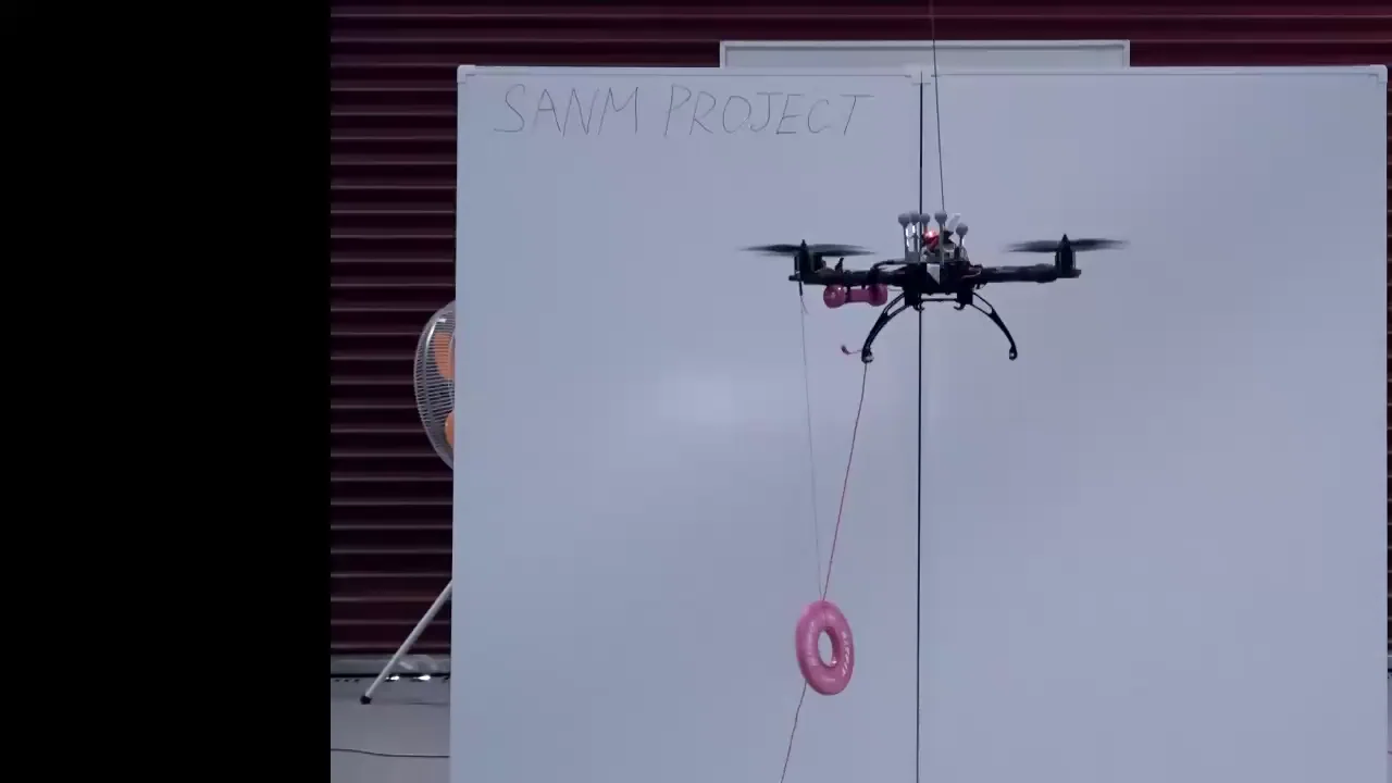
These two demonstrations provide a visual overview of the framework and hardware validation before the detailed geometry, stability analysis, and experiment-by-experiment discussion.

Framework & flight

Wind & impact testbed

Geometry first

The controller operates directly on the rotation manifold. No Euler-angle chart and no quaternion double coverage are required.

Attitude kinematics and disturbed dynamics

The quadrotor attitude is a rotation matrix

$$ \mathrm{SO}(3)= \left\{ R\in\mathbb{R}^{3\times3} \;\middle|\; R^\top R=I,\;\det(R)=1 \right\}. $$

With body angular velocity $\Omega$, inertia tensor $J$, commanded moment $M$, and an acceleration-level rotational disturbance $\phi_R$, the dynamics are

$$ \dot R=R[\Omega]_\times, \qquad \dot\Omega= J^{-1}\!\left(M-[\Omega]_\times J\Omega\right)+\phi_R. $$

Here $[\,\cdot\,]_\times:\mathbb{R}^3\to\mathfrak{so}(3)$ is the skew-symmetric map satisfying $[a]_\times b=a\times b$.

When the inertia is unknown, the gyroscopic term cannot be canceled explicitly. The paper absorbs it together with external effects into a universal disturbance at the acceleration level:

$$ \dot\Omega=J^{-1}M+\phi_R(J,\Omega). $$

This formulation lets the same neural branch identify aerodynamic effects, payload-induced coupling, inertia mismatch, and other continuous unknown accelerations within its compact approximation region.

Quadrotor test platform with body axes, inertia uncertainty, and time-varying disturbance annotation — The physical system used in the study. The body-fixed frame $\mathcal B=\{\vec b_1,\vec b_2,\vec b_3\}$ is attached to the vehicle; an off-center mass creates inertia uncertainty and a suspended payload generates time-varying disturbance moments.

Coordinate-free tracking errors

For desired attitude $R_d$ and desired angular velocity $\Omega_d$, the geometric errors are

$$ e_R= \frac{1}{2} \left(R_d^\top R-R^\top R_d\right)^\vee, $$$$ e_\Omega= \Omega-R^\top R_d\Omega_d, \qquad \Omega_d=(R_d^\top\dot R_d)^\vee. $$

The vee map $(\cdot)^\vee:\mathfrak{so}(3)\to\mathbb{R}^3$ turns the skew-symmetric attitude mismatch into a Euclidean vector. Those three components—and the corresponding three components of $e_\Omega$—are the features seen by SANM.

The scalar attitude configuration error used in the stability proof is

$$ \Psi_R(R,R_d)= \frac{1}{2}\operatorname{tr}\!\left(I-R_d^\top R\right), $$

with the local quadratic bounds

$$ \frac{1}{2}\|e_R\|^2 \leq \Psi_R \leq \frac{1}{2-\psi_R}\|e_R\|^2, \qquad 0\lt\psi_R\lt2. $$

The domain $0\lt\Psi_R\lt2$ covers almost all of $\mathrm{SO}(3)$; the excluded points correspond to the unavoidable $180^\circ$ attitude ambiguity.

From one mapping to three slices

SANM decomposes the inverse identification problem along the roll, pitch, and yaw body axes, then places two complementary online learners in every shared subspace.

Start with the six-dimensional rotational error vector

$$ E_R= \begin{bmatrix}e_R^\top & e_\Omega^\top\end{bmatrix}^{\!\top} =\mathcal S(M_d,J,\phi_R)\in\mathbb{R}^6. $$

Within a compact operating region, the paper assumes a local pseudo-inverse. The sliceability hypothesis decomposes that relationship as

$$ \mathcal S^\dagger(E_R)= \bigoplus_{j=1}^{3} \mathcal S_j^\dagger \left(e_R^{[j]},e_\Omega^{[j]}\right). $$

SANM then realizes the $j$-th submapping as

$$ \left( \bar J^{[j]},\bar\phi_R^{[j]} \right)=\mathcal S_j^{AN} \left( M_d^{[j]},e_R^{[j]},e_\Omega^{[j]} \right), \qquad j\in\{1,2,3\}. $$

01 · $\vec b_1$

Roll slice

$x_{R1}=[e_R^{[1]},e_\Omega^{[1]}]^\top$

Outputs $\bar J^{[1]}$ and $\bar\phi_R^{[1]}$

02 · $\vec b_2$

Pitch slice

$x_{R2}=[e_R^{[2]},e_\Omega^{[2]}]^\top$

Outputs $\bar J^{[2]}$ and $\bar\phi_R^{[2]}$

03 · $\vec b_3$

Yaw slice

$x_{R3}=[e_R^{[3]},e_\Omega^{[3]}]^\top$

Outputs $\bar J^{[3]}$ and $\bar\phi_R^{[3]}$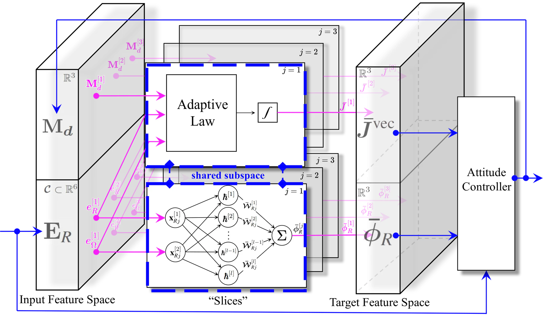

Detailed Sliced Adaptive-Neuro Mapping structure with three axis-wise adaptive law and neural network slices — The high-dimensional mapping is decomposed into three axis-wise slices. In each shared subspace, an adaptive-law slice estimates an effective principal inertia and an RBF-network slice estimates the unknown rotational disturbance.

Learner A — bounded inertia adaptation

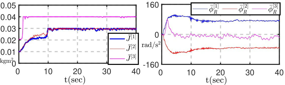
The adaptive branch estimates an effective principal inertia $\bar J^{[j]}$ for each axis. Its reciprocal-form estimation error is

$$ \widetilde J_j= \frac{1}{J^{[j]}}- \frac{1}{\bar J^{[j]}}. $$

Away from the imposed upper boundary, the nominal update is

$$ \dot{\bar J}^{[j]}= -\frac{(\bar J^{[j]})^2}{\eta_j} \left(e_\Omega^{[j]}+c_Re_R^{[j]}\right)M_d^{[j]}. $$

At the prescribed bound $J_j^{\max}$, a pull-back branch replaces outward motion. This keeps the inertia estimate positive and bounded while preserving the cancellation needed in the Lyapunov derivative. The parameter $1/\eta_j$ sets the adaptation rate independently for each axis.

Learner B — shallow RBF disturbance identification

Each neural slice is a $2$-$l$-$1$ radial-basis-function network:

$$ x_{Rj}= \begin{bmatrix} e_R^{[j]}\\ e_\Omega^{[j]} \end{bmatrix} \in\mathbb{R}^{2}, \qquad \phi_R^{[j]}=W_{Rj}^{\top}h(x_{Rj})+\epsilon_{Rj}. $$

The $k$-th Gaussian basis unit is

$$ h^{[k]}(x_{Rj})= \exp\!\left( -\frac{\|x_{Rj}-c_{kj}\|^2}{2b_{kj}^{2}} \right), $$

and the online disturbance estimate is

$$ \bar\phi_R^{[j]}= \bar W_{Rj}^{\top}h(x_{Rj}). $$

The Lyapunov-designed nominal weight update is

$$ \dot{\bar W}_{Rj}^{\mathrm{nom}}= \gamma_{Rj} \left(e_\Omega^{[j]}+c_Re_R^{[j]}\right) h(x_{Rj}). $$

The approximation error separates into weight-estimation error and an irreducible optimal residual:

$$ \phi_R^{[j]}-\bar\phi_R^{[j]}= \widetilde W_{Rj}^{\top}h(x_{Rj})+ \varpi_R^{[j]}, \qquad \widetilde W_{Rj}=W_{Rj}^{*}-\bar W_{Rj}. $$

When $\|\bar W_{Rj}\|$ reaches its prescribed boundary and the nominal update points outward, projection removes the radial component:

$$ \dot{\bar W}_{Rj}= \left( I- \frac{\bar W_{Rj}\bar W_{Rj}^{\top}} {\bar W_{Rj}^{\top}\bar W_{Rj}} \right) \dot{\bar W}_{Rj}^{\mathrm{nom}}. $$

A small error dead zone suppresses bias-driven weight drift near equilibrium. In the reported implementation, an observed bias-induced attitude-error offset of approximately $0.0003$ motivated a dead-zone threshold of $0.0005$.

SANM-augmented geometric control

SANM does not replace the geometric controller. It acts as a feedforward compensator that supplies axis-wise inertia and disturbance estimates to a familiar geometric PD backbone.

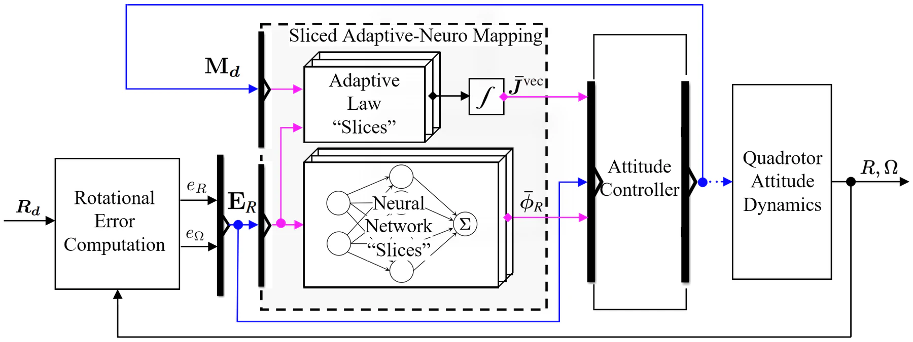
Closed-loop SANM augmented geometric attitude control architecture — Desired and measured attitudes first produce the intrinsic error vector. SANM maps that error into inertia and disturbance estimates, the controller composes the desired moment, and the measured attitude closes the loop.

For body axis $j$, the desired moment is

$$ \begin{aligned} M_d^{[j]}=\bar J^{[j]}\Big(& -k_Re_R^{[j]} -k_\Omega e_\Omega^{[j]}\\ &-\left([\Omega]_\times R^\top R_d\Omega_d\right)^{[j]} +\left(R^\top R_d\dot\Omega_d\right)^{[j]}\\ &-\bar\phi_R^{[j]} +\left(J^{-1}[\Omega]_\times J\Omega\right)^{[j]}_{\text{if }J\text{ is known}} \Big). \end{aligned} $$

If $J$ is known, the gyroscopic term is compensated explicitly. If $J$ is unknown, that term is omitted from the model-based path and absorbed into the universal disturbance learned by the neural slices.

One online control cycle

01
Measure & map
Update $e_R$, $e_\Omega$, $\Omega_d$, and $\dot\Omega_d$ from the current and desired rotations.
02
Adapt inertia slices
Update $\{\bar J^{[j]}\}_{j=1}^{3}$ with the bounded, axis-wise adaptive laws.
03
Evaluate neural slices
Evaluate the RBF bases, update projected weights, and obtain $\{\bar\phi_R^{[j]}\}_{j=1}^{3}$.
04
Compose moment
Compute the three components $\{M_d^{[j]}\}_{j=1}^{3}$ of the desired body moment.
05
Actuate
Send the desired moment to the motor-allocation layer and repeat at the next $2.5$ ms step.

No offline dataset is required. The weights, inertia features, and disturbance features evolve online inside the flight-control loop.

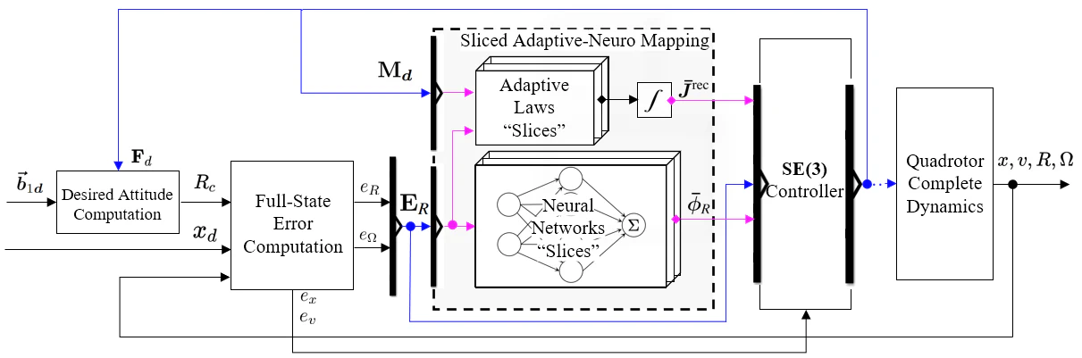
From $\mathrm{SO}(3)$ attitude to $\mathrm{SE}(3)$ flight

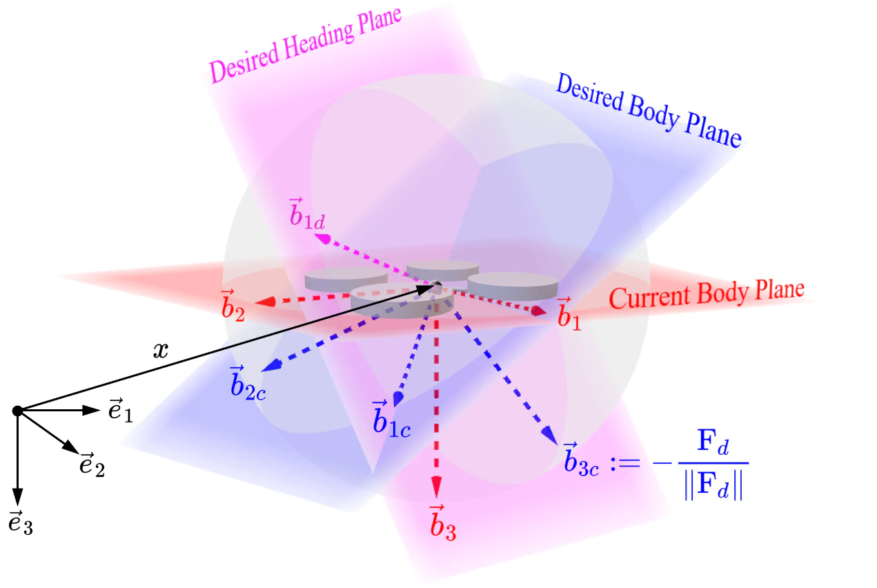
The attitude loop remains compatible with a complete geometric position controller. A desired resultant force $F_d$ defines the commanded body-$z$ direction, while a desired heading $\vec b_{1d}$ completes the commanded attitude frame $R_c=[\vec b_{1c},\vec b_{2c},\vec b_{3c}]$:

$$ \vec b_{3c}=-\frac{F_d}{\|F_d\|}, \qquad \vec b_{2c}=\frac{\vec b_{3c}\times\vec b_{1d}} {\|\vec b_{3c}\times\vec b_{1d}\|}, \qquad \vec b_{1c}=\vec b_{2c}\times\vec b_{3c}. $$

The attitude reference is then set to $R_d\leftarrow R_c$. SANM augments the rotational loop while the translational controller continues to generate $F_d$, which is why the same module can be used in the SITL and real-flight studies.

Quadrotor force, moment, position, velocity, attitude, and angular velocity model on SE3 — The complete rigid-body model couples translational motion in $\mathbb R^3$ with rotational motion on $\mathrm{SO}(3)$.

Construction of the commanded attitude frame from desired force and heading — The position controller supplies a desired force direction; the geometric construction produces a valid commanded rotation for the SANM-augmented attitude loop.

Stability and convergence

The adaptive laws are chosen to cancel parameter-error cross terms in a composite Lyapunov derivative. What remains is an exponential-decay inequality plus a bounded approximation residual.

Rotational error dynamics exposed by SANM

After compensation, an axis-wise representation of the error dynamics is

$$ \begin{aligned} \dot e_\Omega^{[j]}= &-k_Re_R^{[j]}-k_\Omega e_\Omega^{[j]} +\widetilde J_jM_d^{[j]}\\ &+\widetilde W_{Rj}^{\top}h(x_{Rj}) +\varpi_R^{[j]} +\left(J^{-1}\Delta_M\right)^{[j]}. \end{aligned} $$

Here $\Delta_M=M-M_d$ is the moment-allocation deviation and $\varpi_R$ is the optimal neural approximation residual.

Composite Lyapunov function

The proof uses

$$ \begin{aligned} \mathcal V_R= k_R\Psi_R+ \sum_{j=1}^{3}\Bigg( &\frac{1}{2}\left(e_\Omega^{[j]}\right)^2 +c_Re_R^{[j]}e_\Omega^{[j]}\\ &+\frac{\eta_j}{2}\widetilde J_j^2 +\frac{1}{2\gamma_{Rj}} \widetilde W_{Rj}^{\top}\widetilde W_{Rj} \Bigg). \end{aligned} $$

With the adaptive updates above, the key inequality becomes

$$ \dot{\mathcal V}_R \leq -z_R^\top\mathcal M_Rz_R+C_R \leq -2\beta\mathcal V_R+C_R, $$

where

$$ z_R= \begin{bmatrix} \|e_R\|\\ \|e_\Omega\| \end{bmatrix}, \qquad \mathcal M_R= \begin{bmatrix} \frac{k_Rc_R}{2} & -\frac{k_\Omega c_R}{2}\\ -\frac{k_\Omega c_R}{2} & \frac{k_\Omega-c_R}{2} \end{bmatrix}, $$

and

$$ C_R= \frac{c_R\left(\varepsilon_R+\frac{\varepsilon_M}{\lambda_{\min}(J)}\right)^2}{2k_R} + \frac{\left(\varepsilon_R+\frac{\varepsilon_M}{\lambda_{\min}(J)}\right)^2}{2(k_\Omega-c_R)}. $$

A sufficient condition for $\mathcal M_R\succ0$ is

$$ c_R\lt \min\left\{ \frac{k_Rk_\Omega}{k_\Omega^2+k_R}, \sqrt{k_R}, \sqrt{\frac{2k_R}{2-\psi_R}}, k_\Omega \right\}. $$

This exposes the practical meaning of the proof: better function approximation and more accurate moment allocation reduce $C_R$, which contracts the guaranteed residual region.

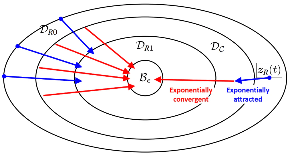
Nested convergence regions

The almost-global claim is subject to the stated initial error and angular-rate conditions. In compact form, the proof starts from

$$ \mathcal D_{R0}=\left\{ \begin{aligned} &0\lt\Psi_R(0)\lt2,\\ &\|e_R(0)\|=\sqrt{\Psi_R(0)\left(2-\Psi_R(0)\right)}\lt1,\\ &\|e_\Omega(0)\|^2\lt k_R\left(2-\Psi_R(0)\right)-\frac{c_R^2}{2} \end{aligned} \right\}. $$

$\mathcal D_{R0}$Almost-global initial setSubject to the stated attitude-error and angular-rate bounds; exact $180^\circ$ ambiguity excluded

$\mathcal D_{R1}$Bounded residual setWorst-case disturbance and approximation bounds

$\mathcal B_\epsilon$Arbitrarily small ballLocal exponential convergence inside $\mathcal D_C$

The almost-global estimate is

$$ \|z_R(t)\| \leq \alpha\|z_R(0)\|e^{-\beta t}+r_1. $$

Once the trajectory enters the compact neural identification region at time $t_1$,

$$ \|z_R(t)\| \leq \alpha\|z_R(t_1)\|e^{-\beta(t-t_1)}+\epsilon, \qquad t\geq t_1. $$

Almost-global attraction

Under the stated initial error and angular-rate conditions, rotational error is exponentially attracted to a bounded residual set.

Local exponential convergence

Inside the identification region, error converges exponentially to an arbitrarily small ball—without persistent excitation.

Compact neural inputs

The slice inputs remain in compact sets, satisfying the prerequisite for universal approximation.

Sampled-data ISpS

The result persists under zero-order hold, finite sampling, and bounded computation delay.

Continuous time · exponential convergence — The continuous proof yields nested exponential convergence regions. The sampled-data extension adds a practical residual caused by finite sampling and bounded computation delay.

Digital implementation · exponential-type ISpS — The continuous proof yields nested exponential convergence regions. The sampled-data extension adds a practical residual caused by finite sampling and bounded computation delay.

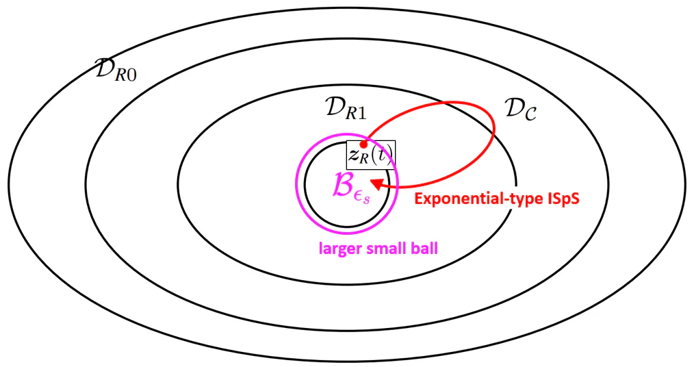
For a sample period $dt$ and computation delay $\tau$, the one-step implementation residual satisfies

$$ 0\leq\Delta_n\leq L(dt^2+dt\,\tau), $$

leading to an exponential-type ISpS estimate

$$ \|z_R(n\,dt)\| \leq \alpha_s e^{-\beta_s n\,dt}\|z_R(0)\|+\epsilon_s. $$

The reported controller uses $dt=0.0025\,\mathrm{s}$ and $\tau\lt dt$, matching the 400 Hz embedded implementation.

Experimental validation

Five progressively harder studies connect the theory to hardware: near-antipodal numerical initialization, wind, impact, high-fidelity physics simulation, and real flight.

01 Numerical02 Wind03 Impact04 Physics05 Flight

Experiment 01 / Numerical simulation

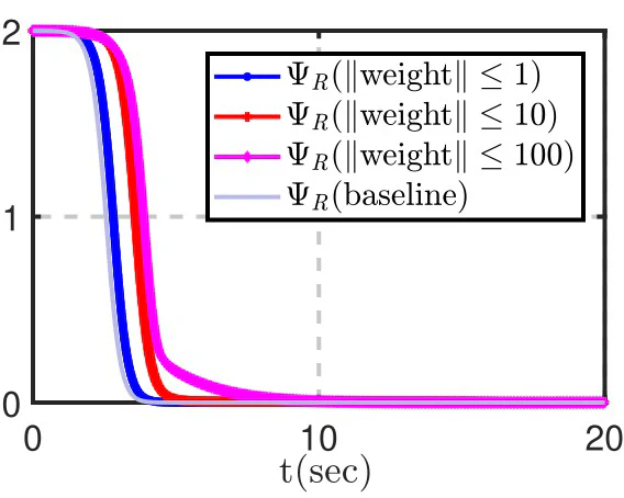
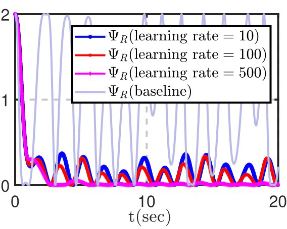
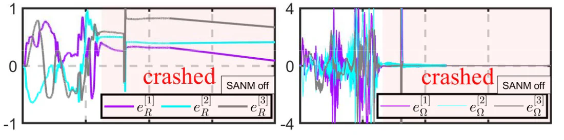
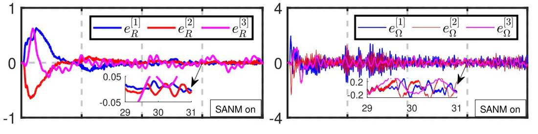
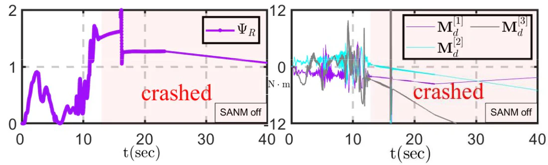
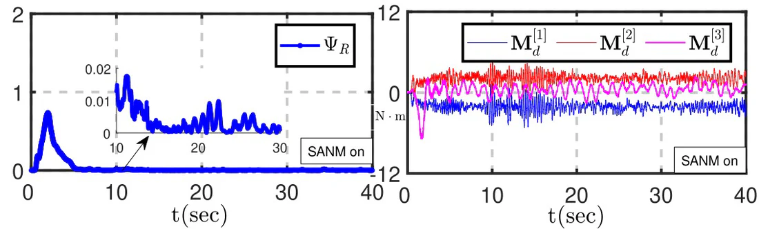
The MATLAB/Simulink study uses fixed-step ODE3 integration at $dt=0.0025$ s. It starts near the antipodal attitude singularity—approximately $179^\circ$, with $\Psi_R(0)=1.9998$—and evaluates both nominal and disturbed unknown-inertia cases.

The injected time-varying disturbance is

$$ \phi_R(t)= \begin{bmatrix} -0.5\sin(\sin(0.2t)t)-3\cos(2t)\\ 0\\0 \end{bmatrix}. $$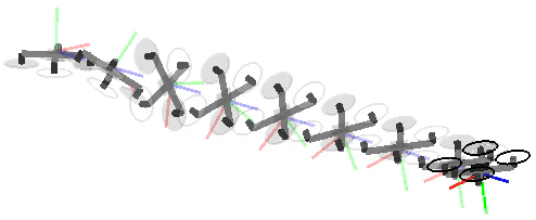

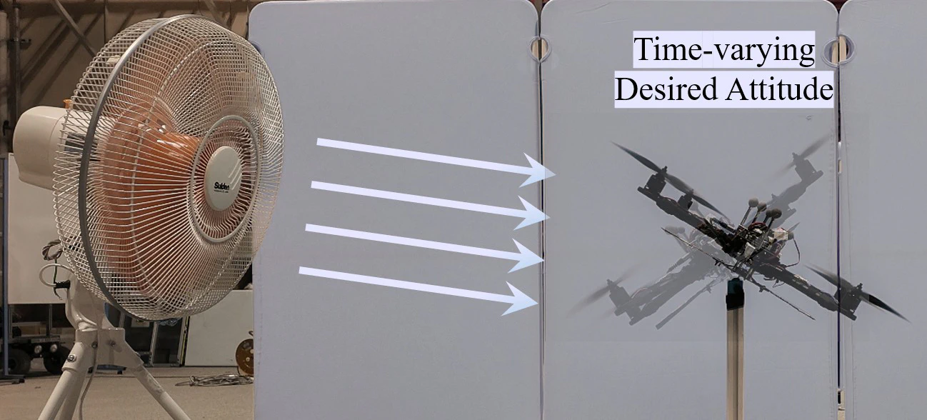
Quadrotor desired and initial attitude configurations separated by approximately 179 degrees — Desired and initial configurations used to test the almost-global domain of attraction.

Unknown inertia · no injected disturbance — Both cases enter the identification region and exhibit the layered convergence behavior predicted by the analysis.

Unknown inertia · time-varying disturbance — Both cases enter the identification region and exhibit the layered convergence behavior predicted by the analysis.

Experiment 02 / Real-world wind disturbance

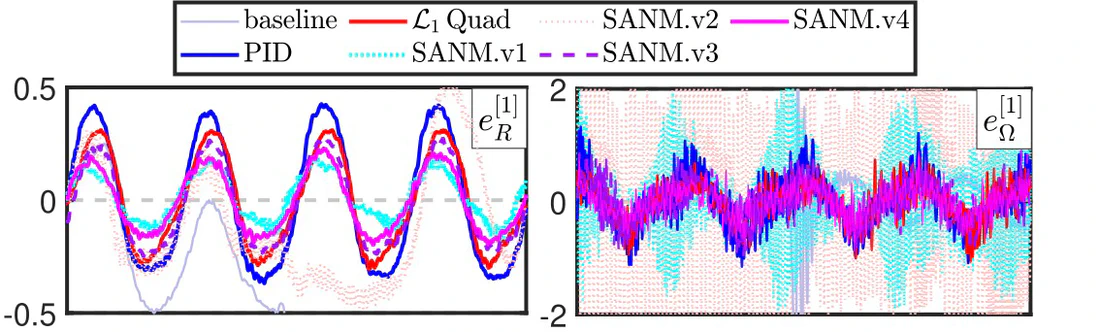
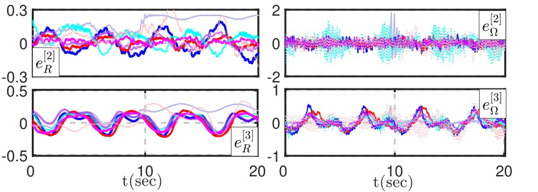
The stationary testbed isolates the attitude loop. Geometric PD, geometric PID, and $\mathcal L_1$ Quad provide reference controllers, all sharing nominal gains $k_R=100$ and $k_\Omega=80$.

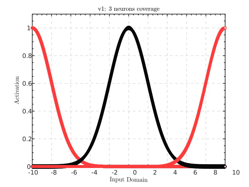
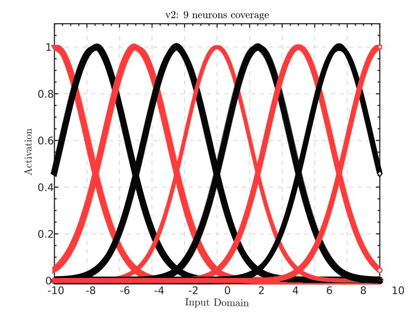
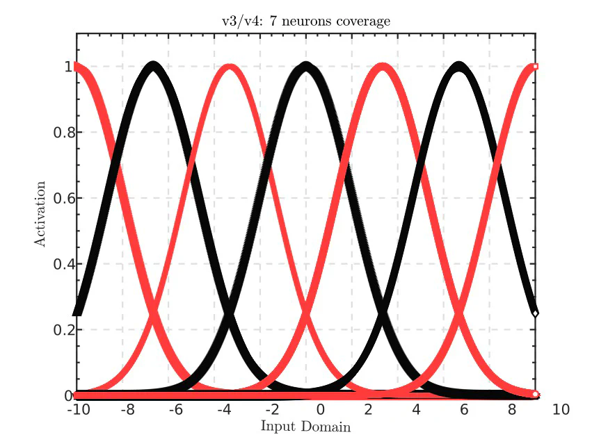
This experiment disables the inertia-adaptation slices to isolate the neural branch. SANM variants use 3, 9, and 7 RBF neurons at learning rates $\{35,35,10\}$; a fourth 7-neuron variant increases the rates to $\{120,120,50\}$. The comparison reveals a practical basis-coverage sweet spot and shows how axis-wise learning rates change the observed residual error ball.

Wind disturbance testbed and plots comparing SANM variants with geometric control benchmarks — Real-world wind-disturbance setup and response comparison. The experiment evaluates network coverage density and learning-rate effects while holding the baseline geometric gains fixed.

3 neurons · sparse coverage — All variants cover the same $[-10,10]$ angular-velocity-error domain with equal basis widths. Changing neuron count changes the density and overlap of the Gaussian basis functions.

9 neurons · excessive overlap — All variants cover the same $[-10,10]$ angular-velocity-error domain with equal basis widths. Changing neuron count changes the density and overlap of the Gaussian basis functions.

Benchmark response comparison — The detailed curves separate the controller benchmark comparison from the two design questions: how densely to cover the slice input domain and how aggressively to adapt each axis.

Coverage density & learning rate — The detailed curves separate the controller benchmark comparison from the two design questions: how densely to cover the slice input domain and how aggressively to adapt each axis.

Experiment 03 / Real-world impact disturbance

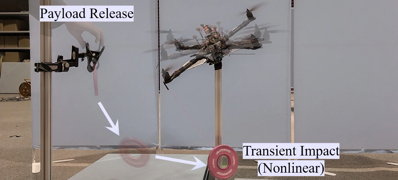
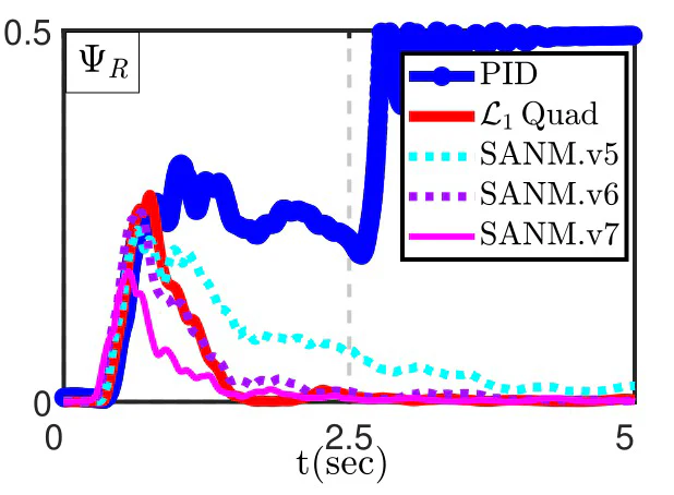
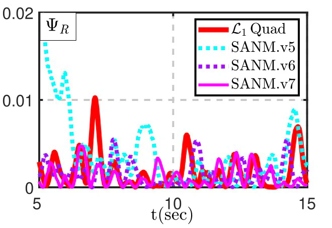
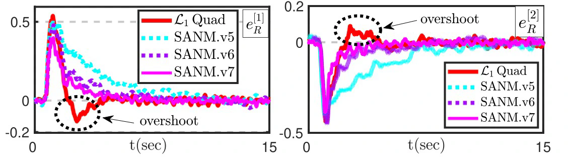
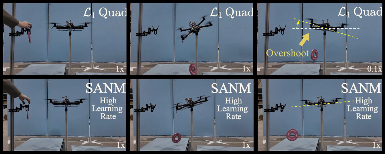
A $0.25$ kg payload is released from one arm, creating a nonlinear impulsive moment. The geometric PID and $\mathcal L_1$ Quad controllers are compared with three 7-neuron SANM variants using learning rates $\{35,35,10\}$, $\{80,80,30\}$, and $\{120,120,50\}$.

In the tested configuration, SANM produces a high-damping, non-overshooting recovery. Increasing the learning rate accelerates the measured recovery and reduces the residual error ball; this is an experimental observation for the reported setup, not a universal no-overshoot claim.

Impact disturbance testbed and response comparison across controllers and SANM learning rates — The impact experiment compares transient spike suppression, recovery speed, and residual steady-state error.

Anti-impact convergence — Increasing the learning rate changes both the transient recovery rate and the measured radius of the post-impact residual error ball.

Residual steady-state error — Increasing the learning rate changes both the transient recovery rate and the measured radius of the post-impact residual error ball.

Impact response curves comparing SANM learning rates with L1 adaptive control — The full-width response plot compares convergence rates and makes the overshoot difference visible.

Supplementary comparison of SANM and L1 adaptive control under impact disturbance — Supplementary transient comparison highlighting the measured high-damping response of SANM under the payload-release disturbance.

Experiment 04 / Gazebo Harmonic physics simulation

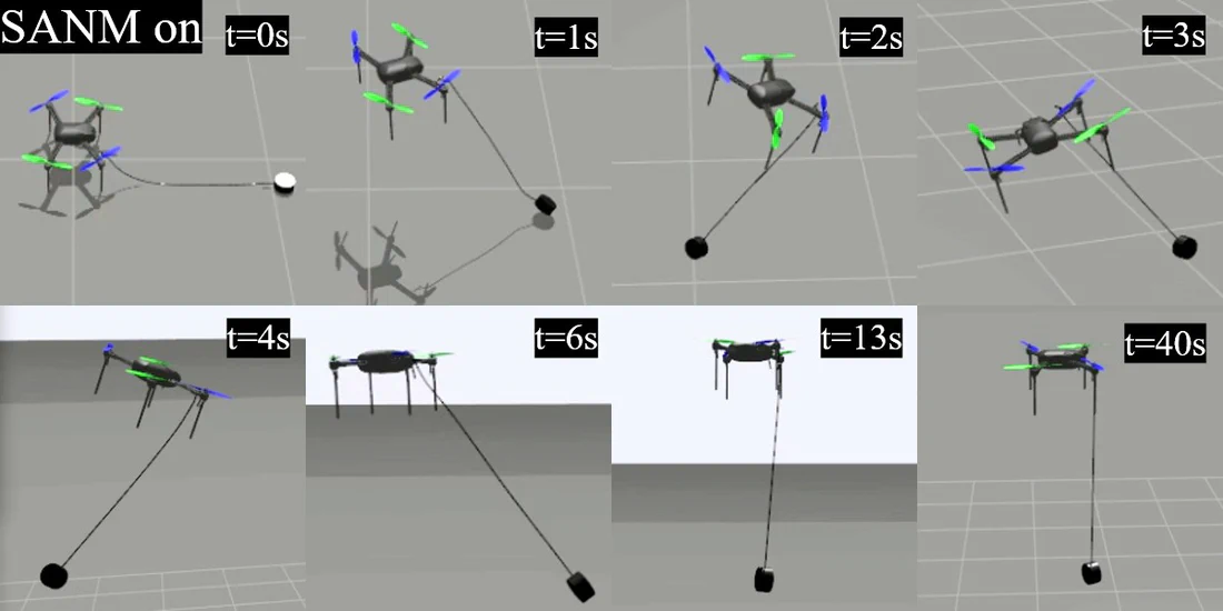
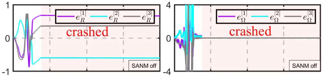
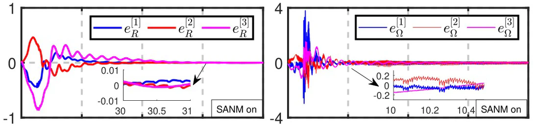
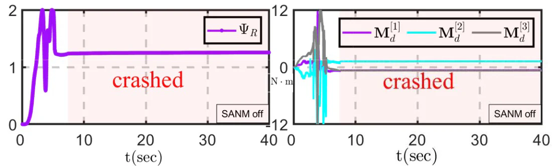
SANM is integrated into the complete $\mathrm{SE}(3)$ position-and-attitude controller inside ArduPilot SITL and Gazebo Harmonic. The 400 Hz loop includes sensor noise, motor delay, and an off-center cable-suspended payload.

The modeled platform uses

$$ m=1.6\,\mathrm{kg},\qquad m_p=0.25\,\mathrm{kg},\qquad m_c=0.02\,\mathrm{kg}, $$$$ J=10^{-2}\operatorname{diag}(1.1,2.0,2.3)\;\mathrm{kg\,m^2}. $$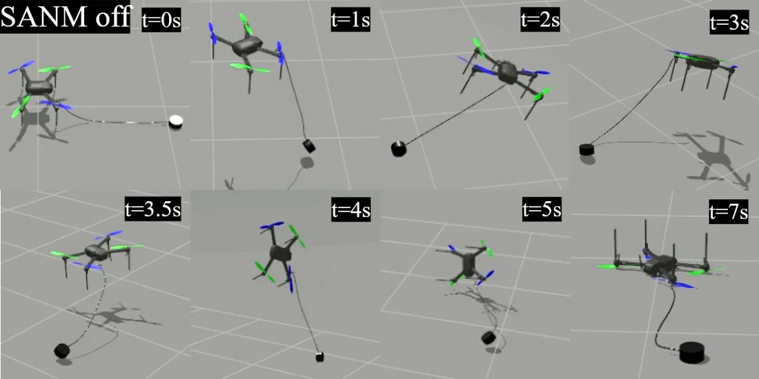

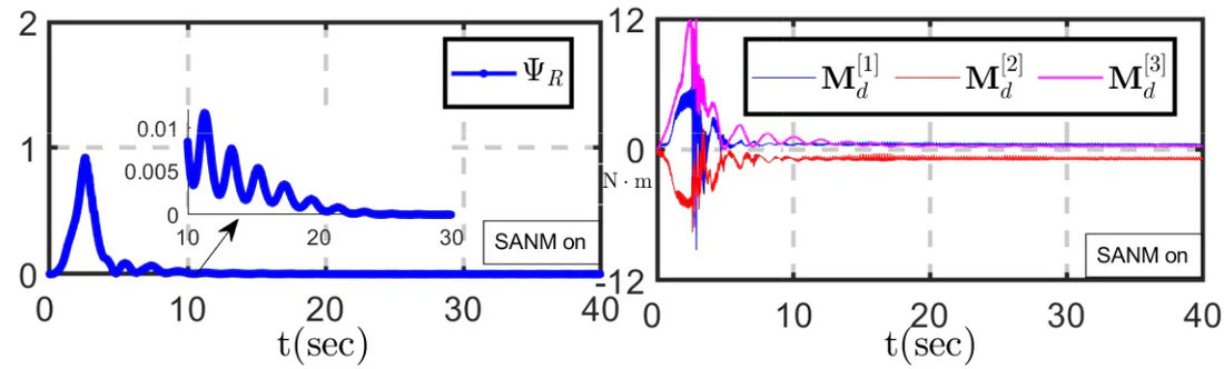
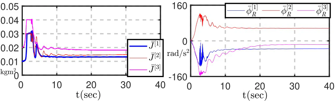
Baseline · SANM off — Controlled comparison with all settings held fixed except activation of the SANM feedforward compensator.

Proposed · SANM on — Controlled comparison with all settings held fixed except activation of the SANM feedforward compensator.

SANM off · attitude and rate errors — The separated state-error plots preserve readable axes and legends instead of compressing the experiment into a paper-sized multi-panel image.

SANM on · attitude and rate errors — The separated state-error plots preserve readable axes and legends instead of compressing the experiment into a paper-sized multi-panel image.

SANM off · configuration error & moment — Configuration-error and commanded-moment histories show how the feedforward estimates alter the closed-loop response.

SANM on · configuration error & moment — Configuration-error and commanded-moment histories show how the feedforward estimates alter the closed-loop response.

Online inertia and rotational disturbance estimates in the Gazebo physics simulation — Real-time inertia-feature and disturbance-feature estimates produced during the high-fidelity simulation.

Experiment 05 / Real-world flight

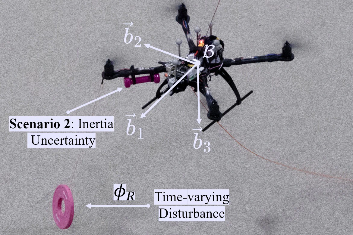
The final experiment transfers the same architecture to a motion-capture flight environment. Three five-neuron networks require only $3\times5=15$ calls to expf() per cycle. An additional off-center $0.25$ kg dumbbell and a suspended $0.25$ kg payload place nearly $800$ g of load on a single rotor.

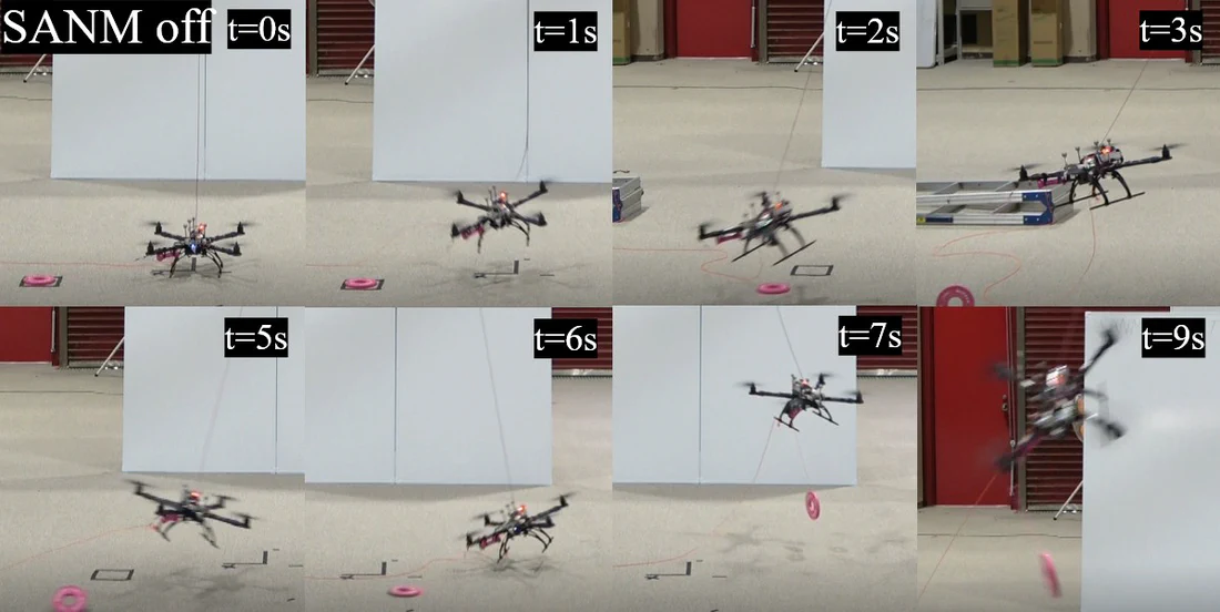
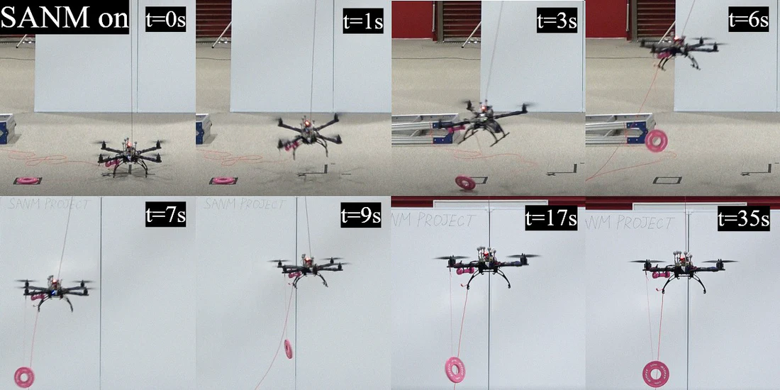
Online SANM estimates recorded during the real flight experiment — Onboard SANM outputs during the real-flight experiment, showing behavior consistent with the physics simulation.

Embedded deployment

The complete learning-and-control loop runs on the flight controller itself—without a companion GPU, Jetson board, or ground-computer inference path.

400HZ

online adaptation inside the ArduPilot 4.6 control loop

Processor: STM32H750 · 480 MHz
Memory: 255.2 kB · 24.9% RAM
Average CPU: 77.2%
Peak CPU: 81.2%
Neural compute: 15 expf() evaluations / cycle
Training data: None · adaptation is online

What the result means

Structural interpretability: each learned quantity has an axis, a defined input, a bounded parameter set, and a visible role in the control law.
Flexible compute: slices can be independently enabled, disabled, or assigned different basis coverage and learning rates.
Theory-to-firmware continuity: the sampled-data result explicitly accounts for zero-order hold, the $2.5$ ms sampling period, and bounded delay.
Extensibility: the same subspace-sharing idea naturally suggests a 12-slice $\mathrm{SE}(3)$ design covering translational and rotational loops.

Paper and citation

PaperRead the full manuscript DOIIEEE/ASME TMECH record NavigationReturn to the top

Cite this work

T. Gao, M. Izumita, K. Tomita, and A. Kamimura, “A Sliced Learning Framework for Online Disturbance Identification in Quadrotor SO(3) Attitude Control,” IEEE/ASME Transactions on Mechatronics, 2026.